License Plate Detection without Machine Learning
In this article, we'll share a simple, yet effective method on how to detect & isolate vehicle registration plate at Real-time without relying on heavy deep-learning techniques or pre-trained models. Just standard image processing routines already implemented in most computer vision libraries out there just like OpenCV or SOD.
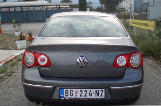
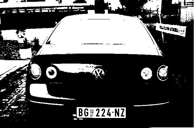
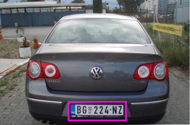
The basic idea for isolating a license plate is to apply a series of morphological image processing algorithms until a potential bounding box is extracted. Keep-in mind that detection is different from recognition which involve optical character recognition on the bounding box output we are going to detect in order to identify the registration plate in question.
For our implementation, we'll be using the SOD embedded computer vision library. For those not familiar with this library, SOD is an open source, modern cross-platform computer vision and machine learning software library that expose a set of APIs for deep-learning, advanced media analysis & image processing including real-time, multi-class object detection and model training on embedded systems with limited computational resource and IoT devices. The project homepage is located at sod.pixlab.io.
Back to our plate detection method. The following are the required steps including the mandatory image processing routines with their proper code implementation we are going to use in order to isolate a license plate in a given image or video frame:
Image or video frame acquisition.
Grayscale colorspace conversion via sod_grayscale_image().
Noise reduction via sod_gaussian_noise_reduce().
Image/frame thresholding via sod_threshold_image().
Canny edge detection via sod_canny_edge_image().
Dilation loop via sod_dilate_image().
Connected component labeling (i.e BLOB detection) via sod_image_find_blobs().
Discard regions of non interest and keep the one that satisfy our requirements using a simple filter callback.
Optionally, crop or draw a bounding box on the target region and start the optical character recognition process on this region.
We'll tackle each step in details now. The fully working code is listed below and can be consulted at the SOD Github repository or the samples page. Just compile the C file with the SOD sources to generate the executable.
Image acquisition & Grayscale colorspace conversion.
The first step is to acquire a video frame from the target video stream such as CCTV or even your smartphone camera. Most modern operating systems offer a low level video capture API for such kind of task and each has its own calling convention. Fortunately, OpenCV do offer an abstraction layer with its CvCapture interfaces that let you capture video frames relatively easily without going too much deep.
For the sake of simplicity here, we'll stick with static images since there is virtually no difference at the processing stage between a video frame and a static image.
Input Picture.

Grayscale Output.
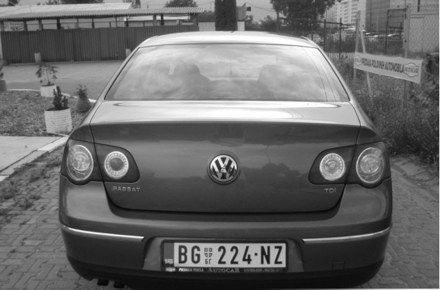
A grayscale (or graylevel) image is simply one in which the only colors are shades of gray. Grayscale images are very common and entirely sufficient for many tasks such as face detection and so there is no need to use more complicated and harder-to-process color images.
There are two methods to convert to grayscale from the RGB/BGR colorspace. Both has their own merits and demerits. The methods are: Average method and Weighted method. You are invited to take a look at the Tutorialpoint page for additional information on the RGB/BGR to Grayscale colorspace conversion.
The gist nearby load a target image from disk (Video capture is omitted for simplicity) and convert the input image to the grayscale colorspace.
Noise Reduction
The second step is to reduce noise from the output grayscale image. There are various techniques for noise removal. The Wikipedia article is a good starting point for your research. In our case, we'll stick with the sod_gaussian_noise_reduce() interface which is not called directly but rather inside the canny edge detection routine as we'll see later.
Basically put, the process is to apply a 5x5 Gaussian convolution filter, shrinks the image by 4 pixels in each direction using a Gaussian filter. This works only on grayscale images which is nice because our image is already converted to that colorspace in the previous step.
Image Thresholding
Thresholding is a technique for dividing an image into two (or more) classes of pixels, which are typically called "foreground" and "background". In our case, we'll use fixed thresholding to obtain a binary image from the grayscale input via sod_threshold_image(). After processing, the output image should look like the following:
Grayscale Input.

Thresholded Image.
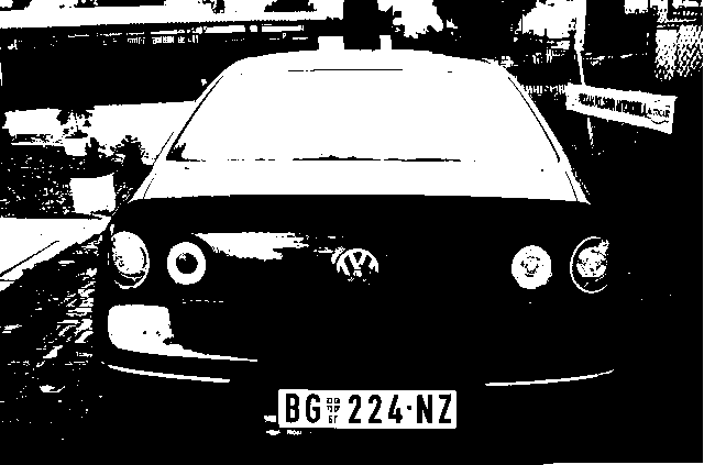
The output is a Binary image whose pixels have only two possible intensity value: Black or White. The gist below highlight this operation. We'll use the canny operator now on this binary image to isolate some potential edges.
Canny Edge Detection
The Canny edge detector is a popular edge detection algorithm. It was developed by John F. Canny in the 80s. It is considered as the ultimate edge detector. You get clean, thin edges that are well connected to nearby edges as shown in the picture below. The sod_canny_edge_image() interface implements the Canny edge operator which expect as its input a grayscale or binary image.
Thresholded Image.

Canny Edge Output.
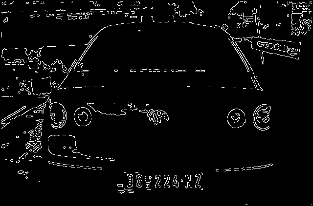
Like thresholding, the output is also a binary image. However, with the canny operator, each region is now completely isolated from each other and potential license plate candidates (i.e. Bounding boxes coordinates) can already be searched for using the Connected Component Labeling (CCL) algorithm as we'll see later. Let's make this task even easier for CCL using a last simple morphological operation: dilation.
Image Dilation Loop
Dilation is a basic morphological operator that is typically applied to binary images like the one obtained from the previous step. The basic effect of the operator on a binary image is to gradually enlarge the boundaries of regions of foreground pixels (i.e. white pixels, typically). Thus areas of foreground pixels grow in size while holes within those regions become smaller. The dilation output is clearly seen below.
Canny Edge Input.

Dilation Loop Output.
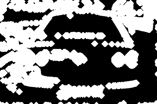
Dilation is applied 12 times here via sod_dilate_image(), hence called dilatation loop. Clearly, the license plate region is completely isolated now having an identifiable rectangular shape. We can use this information to discard region of non interest and keep the one that satisfy our requirements (i.e. rectangular shape with a specific height & width) while performing Connected Component Labeling in the next phase.
Connected Component Labeling
Now that each region is completely isolated from each other, we can apply a very interesting algorithm named Connected Component Labeling or CCL for short. Connected components labeling scans an image and groups its pixels into components based on pixel connectivity, i.e. all pixels in a connected component share similar pixel intensity values and are in some way connected with each other. Once all groups have been determined, each pixel is labeled with a graylevel or a color (color labeling) according to the component it was assigned to.
Dilation Loop Input.

Isolated blocs after CCL (without filtering).
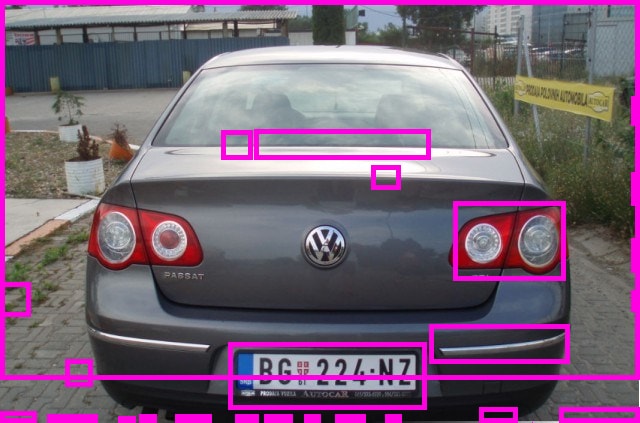
Extracting and labeling of various disjoint and connected components in an image is central to many automated image analysis applications. We can clearly now discard each bloc that does not looks like a rectangular box and keep the one that we can easily identify as a potential license plate using a simple filter callback.
CCL is performed on line 81 via sod_image_find_blobs(). This interface accept a very useful optional parameter which is a user supplied callback that can be used to discard any bloc region that do not satisfy our requirement such as rectangular shape, width and so forth. The filter callback is discussed in the next and last section.
Filter Callback
A filter callback simply put, is a function implemented by the host application that is called by the connected component labeling engine each time a connected blob region is discovered during the matrix (i.e. image pixel data) traversal. The callback is passed as the fourth parameter to sod_image_find_blobs() and it accept two arguments: width and height which hold respectively the width of the discovered blob region and its height. We use these information to discard any region that does not satisfy our requirement. That is, any bloc that does not look like a license plate!
CCL before filtering.

CCL after filtering.

Finally, you'll want to filter the rectangular shapes found that are license plate candidates based on ratio (width / height) and area (width * height). For example, European license plates, had a ratio between 2 and 3.5 and an area of around 5000-7000 pixels while U.S plates have completely different ratio. Obviously this depends on the license plate's shape, the image/frame size, etc.
The gist nearby highlight how a filter callback should be implemented.
Source Code
The full source code presented here in this article is available to consult at the SOD Github repository. You are more than encouraged to compile & link the source file with SOD and play with some samples. The SOD library does also solve object recognition using various Machine Learning approaches. You can find out more information about this via the getting started guide of the library or the samples page for a set working C code. Don't hesitate to reach the SOD developers via their official Gitter channel if you have any question or issue with the code listed here.
Conclusion
The intent of this article is to sensibilize the reader that a machine learning approach is not always the best or first solution to solve some object detection problems. Standard image processing algorithms such as canny edge detection, Hilditch thinning, hough lines detection, etc. when mixed and used properly, are traditionally faster than an ML based approach yet powerful enough to solve those kind of computer vision challenges.